ResNet

标签： Paper CNN

Abstract

通过残差网络的引入，极大的增加了CNN的深度，达到了前所未有的152层，在ILSVRC 2015中获得分类、检测第一名

Introduction

更深的网络层次可以帮助模型获得较好性能，但是也带来一些问题：

• 梯度消失/爆炸
  原因：前面层上的梯度是来自于后面层上梯度的乘乘积。当存在过多的层次时，就出现了内在本质上的不稳定场景，如梯度消失和梯度爆炸。
  Simgmoid容易引发梯度消失，W过大引发梯度爆炸
• degradation的出现
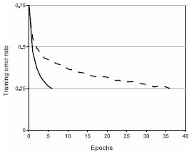
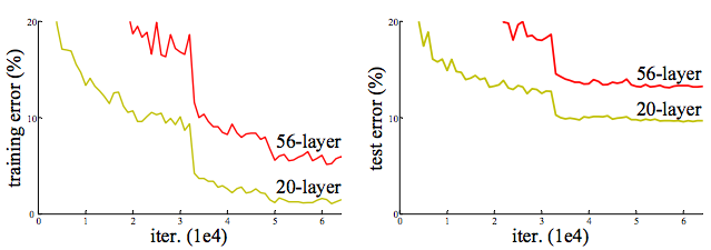
  随着网络加深，train erro反而增加，而不是出现overfitting
  理论上新加入的层如果做identity映射，网络的性能就不会下降，然而实验表明即使是这样的映射也很难被学习
  
• 受此启发，本文提出我们可以帮助网络添加一个shortcut，让网络学习除去identification之外的东西，实验表明最优参数接近于identity，所以由于接近0的参数是比较容易学习的，减轻了网络的学习负担
  

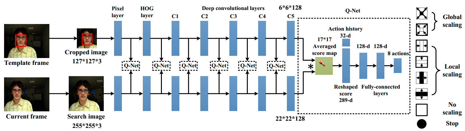
Architecture

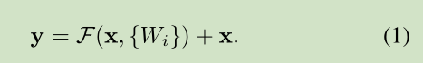
• 公式
  
  只有在维数不匹配时才需要额外的参数Ws（作用在x上），其他情况不会增加参数量
  不仅适用于全连接层，也适用于卷积层

• baseline
  inspired by VGG
  每次feature map减半时，channel加倍

• projection
  当维数不匹配时，可以选择填充0或引入参数，但维数不变时不引入参数（为了减少运算量和存储开销）

• bottleneck Architecture
  
  当网络非常深时，使用上图右半部分的残差块，两个11conv filter用于先把channel降低，在通过33后再拔高channel，这样可以降低计算负担，使之与左边残差块计算量相当

作者还探索了>1000层的网络，但是效果不及100+网络

ICCV2015+ICCV2017 active learning papers

标签： Paper ICCV

ICCV 2017

1. Learning Policies for Adaptive Tracking with Deep Feature Cascades PDF

cmu

使用deep的method效果会好，但速度变慢；而直接用相关滤波的方法，效果没那么好，但速度快。因此作者结合了两种方法，转化为决策问题，提出了一个可以自适应的方法 Early-Stopping Tracker (EAST)，容易track的frame就采用相关滤波即可，而难追踪的frame就继续进行convolution，得到表现好的deep feature。
使用Reinforce Learning训练一个agent，能够在每一层判断是否停止正向传播

将CNN中的future map导入相关滤波

2. Personalized Image Aesthetics pdf

Rutgers University

回归问题，预测用户的美学评分

通用评分预测+个人（内容+属性）网络
通用：cnn euclidean loss
个人：svr
分数及美学属性：cnn fine-tuning
内容属性：分类网络+k-means得到类别 之后fine-tune+soft-max
喂入用户评分与标准分相差较大的样本
3. Hard-Aware Deeply Cascaded Embedding pdf

pku

将网络分为多级，在每一级输出后选择loss较大的样本进入下一级进行训练
4. Adaptive Feeding: Achieving Fast and Accurate Detections by Adaptively
Combining Object Detectors pdf

nju

与1类似，关于object detection

5.Active Learning for Human Pose Estimation pdf
提出了multiple peak entropy， 用于measure uncertainty，

ICCV 2015

1. Context Aware Active Learning of Activity Recognition Model pdf
ucr
Activity Recognition，使用active learning 获得annotation
contribution：基于video中时空的联系，选择最informative的一个activity请求标注
使用CRF

2. Introducing Geometry in Active Learning for Image Segmentation pdf

a novel uncertainty function that combines traditional Feature Uncertainty with Geometric Uncertainty

3. Multi-class Multi-annotator Active Learning with Robust Gaussian Process for
Visual Recognition pdf

multi-class active learning

the problem of active learning with multiple annotators under the condition that multiple annotators may provide noisy labels has not been fully explored

与【1】类似，也是使用reinforce learning的方法选择informative的样本

4.Active Transfer Learning with Zero-Shot Priors:Reusing Past Datasets for Future Tasks pdf
image classification问题
选择svm临界部分数据

Fine-tuning

Joint Fine-Tuning in Deep Neural Networks for Facial Expression Recognition pdf

• 数据量较小，而网络很复杂（参数多，维数高），不足以支撑从0开始训练

Pytorch学习笔记(二)

标签： pytorch

torch.gather

torch.gather(input, dim, index, out=None) → Tensor

如果input是一个n维的tensor，size为 (x0,x1…,xi−1,xi,xi+1,…,xn−1)，dim为i，然后index必须也为n维tensor，size为 (x0,x1,…,xi−1,y,xi+1,…,xn−1)，其中y >= 1，最后输出的out与index的size是一样的。

对于一个三维向量来说：

out[i][j][k] = input[index[i][j][k]][j][k]  # if dim == 0
out[i][j][k] = input[i][index[i][j][k]][k]  # if dim == 1
out[i][j][k] = input[i][j][index[i][j][k]]  # if dim == 2

PIL.Image/numpy.ndarray与Tensor的相互转换

PIL.Image/numpy.ndarray转化为Tensor，常常用在训练模型阶段的数据读取，而Tensor转化为PIL.Image/numpy.ndarray则用在验证模型阶段的数据输出。

我们可以使用 transforms.ToTensor() 将 PIL.Image/numpy.ndarray 数据进转化为torch.FloadTensor，并归一化到[0, 1.0]：

• 取值范围为[0, 255]的PIL.Image，转换成形状为[C, H, W]，取值范围是[0, 1.0]的torch.FloadTensor；
• 形状为[H, W, C]的numpy.ndarray，转换成形状为[C, H, W]，取值范围是[0, 1.0]的torch.FloadTensor。

存储和恢复模型并查看参数

方法一(推荐)：

保存
torch.save(the_model.state_dict(), PATH)
恢复
the_model = TheModelClass(*args, **kwargs)
the_model.load_state_dict(torch.load(PATH))

方法二：

保存
torch.save(the_model, PATH)
恢复
the_model = torch.load(PATH)

nn.module

举例

class TwoLayerNet(torch.nn.Module):
def __init__(self, D_in, H, D_out):
    """
    In the constructor we instantiate two nn.Linear modules and assign them as
    member variables.
    """
    super(TwoLayerNet, self).__init__()
    self.linear1 = torch.nn.Linear(D_in, H)
    self.linear2 = torch.nn.Linear(H, D_out)
def forward(self, x):
    """
    In the forward function we accept a Variable of input data and we must return
    a Variable of output data. We can use Modules defined in the constructor as
    well as arbitrary operators on Variables.
    """
    h_relu = self.linear1(x).clamp(min=0)
    y_pred = self.linear2(h_relu)
    return y_pred

Abstract

进一步加深了网络，在ImageNet 2014中定位和分类任务分别获一二名

Introduction

• ILSVRC-2013 使用了更小的window size和更小的stride。

• 本文使用更小的filter，稳定的增加了网络深度（更多卷积层）

Architecture

基本架构

• 224*224 input 减去均值
• 使用了33和11卷积，保留维度的填充，部分卷积层后跟max-pooling2*2
• 3 fc layer（4096 input） 1 softmax
• 所有激活函数为relu
• LRN因为没有效果而被弃用
  图示
  ![vggNet Architecture][1]
  ![number of parameters][2]
  讨论
  多个33层可以达到77的视野，同时减少了参数数量，增加了非线性
  1*1保持channel数不变，增加了模型能力

Classification Task

与Alex类似，74次迭代后停止

We conjecture that in spite of the larger number of parameters and the greater depth of our nets compared to (Krizhevsky et al., 2012), the nets required less epochs to converge due to (a) implicit regularisation imposed by greater depth and smaller conv. filter sizes; (b) pre-initialisation of certain layers.

初始化：
先使用随机初始化训练较浅网络，使用训练后的结果（前四层和后三层）初始化更深的网络

图片处理：
isotropically-rescaled：各向同性缩放
先缩放为S大小：[256,512]，再随机取区域裁剪为224*224

测试：
缩放为scale Q
将全连接转化为卷积，最后得到1000nn的输出，等效于在scale Q上选取了n*n个位置放入神经网络
节省了计算量

作者：Hao Zhang
链接：https://www.zhihu.com/question/53420266/answer/180001976
来源：知乎
卷积层和全连接层的唯一区别在于卷积层的神经元对输入是局部连接的, 并且同一个通道(channel)内不同神经元共享权值(weights). 卷积层和全连接层都是进行了一个点乘操作, 它们的函数形式相同. 因此卷积层可以转化为对应的全连接层, 全连接层也可以转化为对应的卷积层.
比如VGGNet中, 第一个全连接层的输入是77512, 输出是4096. 这可以用一个卷积核大小77, 步长(stride)为1, 没有填补(padding), 输出通道数4096的卷积层等效表示, 其输出为114096, 和全连接层等价. 后续的全连接层可以用1x1卷积等效替代.
简而言之, 全连接层转化为卷积层的规则是: 将卷积核大小设置为输入的空间大小.这样做的好处在于卷积层对输入大小没有限制, 因此可以高效地对测试图像做滑动窗式的预测. 比如训练时对224224大小的图像得到77512的特征, 而对于384384大小的测试图像, 将得到1212512的特征, 通过后面3个从全连接层等效过来的卷积层, 输出大小是66*1000, 这表示了测试图像在36个空间位置上的各类分数向量. 和分别对测试图像的36个位置使用原始的CNN相比, 由于等效的CNN共享了大量计算, 这种方案十分高效而又达到了相同目的
参考文献
[1]Simonyan, Karen, and Andrew Zisserman. “Very deep convolutional networks for large-scale image recognition.” arXiv preprint arXiv:1409.1556 (2014).
[2]. Lin, Min, Qiang Chen, and Shuicheng Yan. “Network in network.” arXiv preprint arXiv:1312.4400
[3]. Sermanet, Pierre, et al. “Overfeat: Integrated recognition, localization and detection usingconvolutional networks.” arXiv preprint arXiv:1312.6229 (2013).
[4]. Long, Jonathan, Evan Shelhamer, and Trevor Darrell. “Fully convolutional networks forsemantic segmentation.” Proceedings of the IEEE Conference on Computer Vision andPattern Recognition. 2015.
[5]. Fei-Fei Li, Andrej Karpathy, and Justin Johnson. CS231n: Convolutional Neural Networks for Visual Recognition. Stanford. 2016.

Evaluation

![evaluation results][3]
![multi-scale evaluation][4]
![dense&crop evaluation][5]
![convNet fusion evaluation][6]

比GoogLeNet泛化性能更好
[1]: http://upload-images.jianshu.io/upload_images/3232548-bcc2ded7859ee146.png?imageMogr2/auto-orient/strip%7CimageView2/2/w/1240
[2]: http://upload-images.jianshu.io/upload_images/3232548-42a791044eec4ff3.png?imageMogr2/auto-orient/strip%7CimageView2/2/w/1240
[3]: http://upload-images.jianshu.io/upload_images/3232548-0bf25f504335c186.png?imageMogr2/auto-orient/strip%7CimageView2/2/w/1240
[4]: http://upload-images.jianshu.io/upload_images/3232548-5efba64ff7d5c399.png?imageMogr2/auto-orient/strip%7CimageView2/2/w/1240
[5]: http://upload-images.jianshu.io/upload_images/3232548-076a5b039b016b20.png?imageMogr2/auto-orient/strip%7CimageView2/2/w/1240
[6]: http://upload-images.jianshu.io/upload_images/3232548-396bedeb565e428c.png?imageMogr2/auto-orient/strip%7CimageView2/2/w/1240

Abstract

high-resolution 高分辨率

ImageNet Top-1 
对一张图片，如果概率最大的是正确答案，则正确
TOp-5 概率前五正确则正确

AlexNet 
1.2million images 1000classes
Top-1 erro 37.5% 
Top-5 erro 17.0%
60million parameter
5 conv layer + 3 pooling layer
2 ful-con layer
1 softmax layer

no-saturating neurons
使用不挤压输出的激活函数，如relu等，可以减少梯度消失情况的出现

dropout 减少过拟合

Backgroud

• 大规模数据集出现
• CNN有较强模型能力，适于图像处理任务
• GPU对于卷积的优化

Dataset

from ImageNet-2010
256 * 256 缩放+裁剪
预处理：RGB减去分别减去平均值

Achitecture

1. RELU

• 弃用了传统的tanh或是sigmoid，改用$ f(x) = max(0,x) $,大大提高了训练速度
  

图2：采用ReLUs的四层CNN（实线）对CIFAR-10数据集达到25%训练错误率的速度是采用tanh的CNN（虚线）的六倍。每个网络的学习率（learning rate）都是独立选取以使其训练速度最大化，且都没有经过正则化处理。当然，两种CNN的训练时间上的差距依不同架构会有所不同，但采用ReLUs的CNN总是快过用饱和激活函数的CNN。

2. 多GPU训练

• 在两个GPU并行训练
• 俩个GPU只在某些特定层传递数据

3. 归一化

• 从生物神经中受到启发
• 近邻的较大值可以对自身进行抑制

4. overlapping pooling

• 3*3 2步长 减少了过拟合

  4. 整体架构

• 如上图

input    227 * 227 * 3 
conv1    11 * 11 * 3 * 96
active1  55 * 55 * 48 * 2
pool1    27 * 27 * 48 * 2
conv2    5  * 5  * 48 * 128 * 2
active2  27 * 27 * 128 * 2
pool2    13 * 13 * 128 * 2
conv3    3  * 3  * 256 * 192 * 2
active3  13 * 13 * 192 * 2
conv4    3  * 3  * 192 * 192 * 2
active4  13 * 13 * 192 * 2
con5     3  * 3  * 192 * 128 * 2
active5  13 * 13 * 128 * 2
pool5    6  * 6  * 128 * 2
fulc1    6  * 6  * 256 * 4096  
active6-7  2048 * 2
sofmax   1000

Reduce Overfitting

1. 数据增广

训练数据的载入（以及生成）在CPU上进行，与GPU中的训练并行

• 通过对原图进行变换（256256提取出224224）以及水平翻转，训练集增加2048倍
  测试时取五个224*224以及对应水平翻转
• 基于PCA对于每个像素的色彩进行变换，使得物体识别不依赖于色彩

1. 随机失活
   在前两个全连接层使用随机失活，降低神经元之间的依赖性，失活概率0.5
   测试时不进行随机失活，将输出乘以0.5
   收敛速度受到了影响

More Detail

1. w随机初始化，接近0，b在relu层初始化为1，其他为0，以加快收敛
2. 使用随机梯度下降，momentem，weight decay
3. 学习率从0.01开始，逐渐降低，每次loss不减小后除10
4. 120万图片，90次迭代

Pytorch学习笔记(一）

标签 ： pytorch

tensor

x = torh.Tensor(2, 3) #生成一个2*3的tensor

Variable

位于pytorch.autograd中，有data（Tensor类型），grad，grad_fn等属性

#####只有在需要时才使用Variable类型，否则使用numpy或tensor

Function

重写function需要实现forward()与backward(),下面给出

class LinearFunction(Function):
# forward 和 backward 都是 静态方法
@staticmethod
# bias 是个可选参数，有个 默认值 None
# ctx 参数必选，用于保存上下文供backward使用
def forward(ctx, input, weight, bias=None):
    # input，weight 都是 Tensor

    ctx.save_for_backward(input, weight, bias)
    output = input.mm(weight.t())
    if bias is not None:
        output += bias.unsqueeze(0).expand_as(output)
    return output
    # 返回Tensor

# 由于 forward 只有一个返回值，所以 backward 只需要一个参数接收梯度。
@staticmethod
def backward(ctx, grad_output):
    # grad_output 是 Variable 类型。
    # 在开头的地方将保存的 tensor 给 unpack 了
    # 然后给所有应该返回的梯度以 None 初始化。
    # saved_variables 返回的是 Variable！！！
    input, weight, bias = ctx.saved_variables
    grad_input = grad_weight = grad_bias = None

    # needs_input_grad 检查是可选的
    # 返回值的个数需要和 forward 形参的个数（不包含 ctx）一致
    if ctx.needs_input_grad[0]:
        grad_input = grad_output.mm(weight)
    if ctx.needs_input_grad[1]:
        grad_weight = grad_output.t().mm(input)
    if bias is not None and ctx.needs_input_grad[2]:
        grad_bias = grad_output.sum(0).squeeze(0)
    # 梯度的顺序和 forward 形参的顺序要对应。
    return grad_input, grad_weight, grad_bias

Welcome to my blog!